How Multi-Channel Convolution Works

As you probably already know, a single-channel convolution works by sliding a 2D filter, usually smaller than the input matrix, across the height and width dimensions. For every sliding “window”, we then compute the weighted sum. The resulting output is a smaller 2D matrix.
simple convolution
Most of the time, however, we are dealing with tensors that have more than one channel (a colored image for example). Things get even more complicated when we want to have a different number of input and output channels.
We’ll be looking at how to transform an F x F input matrix with M channels into a G x G output matrix with N channels via convolution using a K x K kernel.
This post focuses on the dimensional aspect of convolutions. For a detailed introduction to the applications of CNN, check out this article.
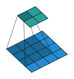
Single Filter Convolution
Assuming zero paddings and a stride of one, a single-channel convolution looks like this:
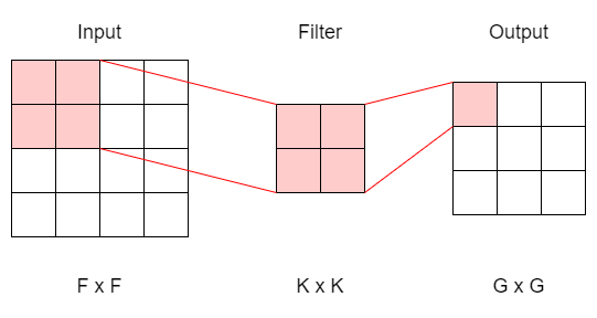
single channel convolution
There is only one filter (K x K), and each time it slides across the input matrix, we compute the weighted sum and compress the information into a single cell on the output matrix. Repeat and we’ll have a G x G final output.
Now if we add in M channels for the input matrix, we’ll also have to add M channels for the filter. Likewise, we can compute the weighted sum across M channels, resulting in the same output dimension as before.
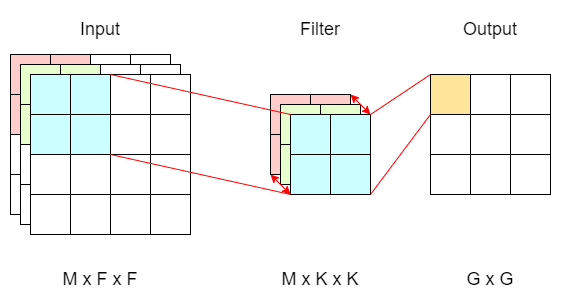
multi channel convolution with M input channels
Note that the filter (now M x K x K) will always have the same number of channels (M) as the input matrix (M x F x F). This way, when we’re calculating the weighted sum, each input channel will have its corresponding kernel.
The resulting output, after passing the input matrix through a single filter, remains 2 dimensional (G x G) regardless of the number of input channels. This is because the filter sums up all the weighted sums across all channels, projecting the final result into a single cell for each sliding window.
We have successfully dealt with multi-channel inputs, next we’ll look at how do we expand our output to N channels.
Multi Filter Convolution
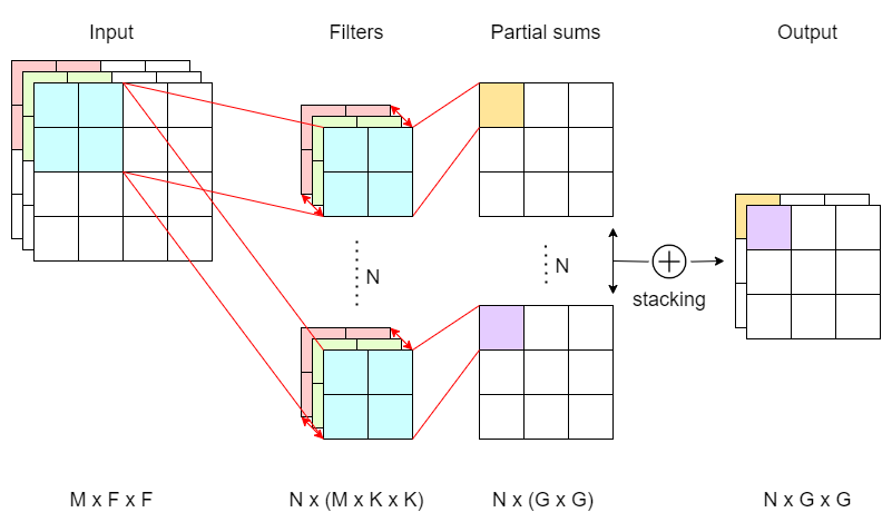
multi-channel convolution with M input channels N output channels
We already know that for each filter we have, we get an output matrix of G x G. The trick to augment our output to any N channels we want is then to have N filters, and this is exactly how multi-channel convolution works under the hood. Instead of just a single filter, we train N filters (M x K x K), and each filter will output a partial sum matrix with a dimension G x G. Finally, we stack all the partial sums, which we should have N of them, to form a final output matrix of N x G x G.
That’s it, now you know how multi-channel convolution works!
Conclusion
Multi-channel convolution works by training N filters, each with dimensions of M x K x K, and stacking the final partial sums, resulting in an N x G x G output matrix.