How Sampling on a Spherical (Polar) Coordinate Can be Biased

Continuing from last week’s discussion on the volume of a hypersphere, we’re going to take a look at how to uniformly sample points on a 3D sphere (also applies to N-dimensional Hyperspheres), and the common pitfall that comes with it.
Let’s say you are building an algorithm that spawns Pokemons at random locations all around the globe for the game Pokemon Go. The first thing you might do is to uniformly sample locations on Earth to spawn your Pokemons. To do so we’ll assume that the Earth is a perfect unit sphere (radius equals 1).
Common Pitfall - Sampling with Spherical Coordinate
Perhaps one of the most intuitive ways to generate this distribution is to uniformly sample from the spherical (polar) coordinate. Only two random variables $\phi \in [0, \pi)$ and $\theta \in [0, 2\pi)$ are needed in this case if we set $\rho = 1$. Here’s the implementation in Python.
N = 10000 # sample count

rho = 1 # constant radius rho

# uniformly sample two random variables from 0 to 2pi
phi = np.random.uniform(low=0, high=np.pi, size=N)
theta = np.random.uniform(low=0, high=2 * np.pi, size=N)
It’s as simple as that. Except if you live in or near the poles, this is what you’re going to see when you pull up the game.

we do not talk about the missing ear.
Too crowded, isn’t it? But didn’t we use uniform sampling?
Let’s visualize the distribution of these critters. Since the random points are on a globe, we’ll have to project it down to 2D.
# convert back to Cartesian coordinate
x = rho * np.sin(phi) * np.cos(theta)
y = rho * np.sin(phi) * np.sin(theta)
z = rho * np.cos(phi)

# plot
fig, (ax1, ax2) = plt.subplots(1, 2, figsize=(11, 5))
fig.suptitle('Sampling with Spherical Coordinate (Biased)')
ax1.scatter(x, y, s=1)
ax1.set_title('top down view')
ax1.set_xlabel('x')
ax1.set_ylabel('y')
ax2.scatter(x, z, s=1)
ax2.set_title('side view')
ax2.set_xlabel('y')
ax2.set_ylabel('z')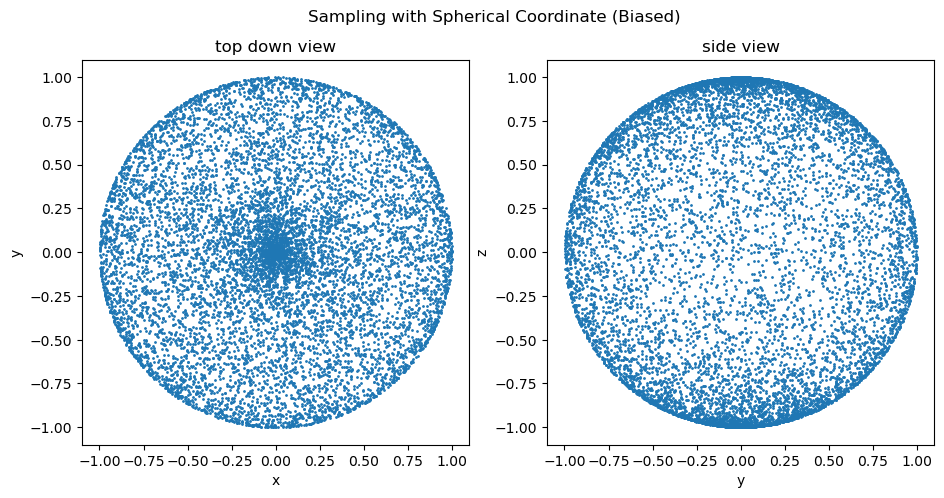
2D projection of a sphere
This is interesting. If the distribution is truly uniform, looking at the sphere from any angle should give us roughly the same picture. However, from our distribution graph, we can see a region of concentrated points at the center of the top-down view, where the poles are supposed to be, while the side view seems relatively sparse in the middle.
So why do the Pokemons love the cold so much?
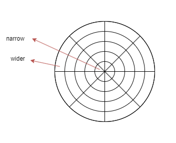
Top-Down view of the Spherical Coordinate
As it turns out, this sampling method in the spherical coordinate isn’t exactly uniform. You can read more about the math behind it here. But in short, think of it this way: Under the spherical (polar) coordinate system, the grid lines are radial. If we were to uniformly distribute the points evenly in these regions cut out by the grid lines as shown above, the regions near the poles will inevitably have a higher density of points than the regions near the equator since the area is smaller.
The Solution - Sampling with Multivariate Normal
Luckily, there’s an easy solution. All we have to do is generate a vector (3D) with a mean of 0 and a standard deviation of 1 — a multivariate normal distribution. This distribution is invariant under any rotations in the 3D space. We can then normalize this vector for the point to be uniformly distributed on the sphere.
D = 3
N = 10000

# sample from gaussian distribution
v = np.random.multivariate_normal(np.zeros(3), np.identity(3), size=N)

# normalize
v = v / np.linalg.norm(v, axis=1, keepdims=True)
Let’s visualize the distribution again.
# Extract Cartesian corrdinate
x, y, z = v[:, 0], v[:, 1], v[:, 2]

# plot
fig, (ax1, ax2) = plt.subplots(1, 2, figsize=(11, 5))
fig.suptitle('Sampling with Multivariate Normal (Uniform)')
ax1.scatter(x, y, s=1)
ax1.set_title('top down view')
ax1.set_xlabel('x')
ax1.set_ylabel('y')
ax2.scatter(x, z, s=1)
ax2.set_title('side view')
ax2.set_xlabel('y')
ax2.set_ylabel('z')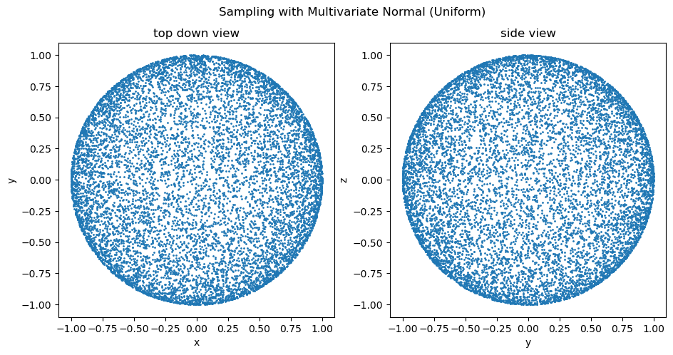
2D projection of a sphere
Yay! Now both the top-down view and the side view look nearly identical — a uniformly distributed sample! This technique also works for hyperspheres of any dimension.