Volume of a Hypersphere (N-Ball) is Weird...

This week I was watching Netflix’s latest sci-fi adaptation of Three Body Problem (SPOILER ALERT). The story revealed how the San-Ti alien race built the Sophon, a supercomputer the size and mass of a single proton, to sabotage the scientific advancement on Earth. While the TV series didn’t dive too deep into the methodology behind it, the novel (strongly recommend!) described how the San-Ti engineers were able to take advantage of the dimensions of these particles. The Sophon was originally a regular proton (11D by default) “unfolded” into a planet-sized 2D plane, which allowed the alien scientists to etch a humongous supercomputer circuit onto its surface. This planet-sized supercomputer proton is then “folded” back into its original form with 11 dimensions, making it virtually impossible to detect since it has the same size and mass as any other proton. How cool is that?
At first thought, most of us probably think that “if it has more dimensions, it must be bigger”. So why exactly is the 2D proton bigger than its 11D counterpart?
Let’s find out.
The N-Ball Problem
For our experiment, we’ll first need a mathematical model.
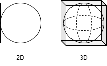
We’ll assume a proton takes the shape of a hypersphere (a ball in N-dimension, or an N-ball). A 2D hypersphere is a circle, and a 3D hypersphere is — you guessed it — a sphere. Anything above we cannot fully visualize with our 3D-wired brain.
Since we are comparing the “size” of the hypersphere, we’ll use its volume in the n-dimension as the main metric. By definition, the volume of something is how much “space” it takes up, for example, the volume of a 2D hypersphere is simply the area of a circle ($\pi r^2$), as for a 3D hypersphere it is the spherical volume ($\frac{4}{3}\pi r^2$).
Nothing crazy so far.
However, the math gets a little complicated in the higher dimensions. You can find a whole list of formulas for the Volume of an N-Ball on Wikipedia, but we won’t dive into the theoretical details here.
Now, applying our hypersphere model to our claim, here we try to find out does a hypersphere in low dimension (e.g. 2D) has a higher volume than a hypersphere in high dimension (e.g. 11D), under a fixed radius?
But does this even make sense?
Let’s first try doing some basic calculations, we’ll assume a unit hypersphere (radius of 1). A 2D unit hypersphere has a volume of $\pi$, and its 3D counterpart has a volume of $\frac{4}{3}\pi$. This tells us that at least in the lower dimensions, the volume of a hypersphere increases as its dimension increases, and it makes sense since we know that for a fixed radius a sphere takes up more space than a flat circle, but this doesn’t quite align with our claim.
What about the volume of a hypercube (cube in N-dimension)? Let’s assume a hypercube with a side length of 2, this way the hypercube will always enclose a unit hypersphere (radius of 1) in the same dimension. It is fairly easy to compute the volume of such a hypercube as it is just $2^n$. The volume of a hypercube increases exponentially as the dimension increases, another counter-example for our claim.
Every calculation we’ve done above seems to suggest that volume should increase with dimensions, but is it really the case? Since this blog is mainly about coding, we’ll attempt to dig up the truth with some good old Monte Carlo simulations.
The Expanding Corners
A hypercube bounding a hypersphere in different dimensions
As mentioned, a hypercube with a side of 2 will always enclose a unit hypersphere in any dimension. These unit hypersphere are the largest hypersphere possible to exist within these hypercubes without overflowing. The volume of these hyperspheres is therefore bounded by the volume of the hypercube $2^n$.
For our simulation, we’ll first sample 1 million random points within the $n$ dimension hypercube with a side length of 2. This is a fairly straightforward process as all we have to do is generate $n$ random points within the interval $[-1, 1]$ 1 million times.
Next, for each point, we can easily tell if it lies within the bounded hypersphere by checking if the Euclidean distance from the point to the origin is greater than the radius 1. For points that lie outside of the hypersphere but within the hypercube, we say that these points sit in the corners. We can then compute the ratio of points that sit in the corners out of all 1 million points. This should give us a good estimation of the percentage of space that belongs to the corners within the hypercube without having to deal with the complex volume formulas.
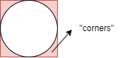
“corners” of a hypercube and hypersphere in 2D
We’ll repeat this simulation across dimensions 1 to 20 and graph the trend.
import numpy as np
from matplotlib import pyplot as plt

N = 20
SAMPLE_SIZE = 1000000

corners_count = []
for n in range(1, N + 1):
    # sample points within hypercube
    pts = np.random.uniform(low=-1, high=1, size=(SAMPLE_SIZE, n))
    # compute percentage that lies in the corners
    corners = np.sum(np.sqrt(np.sum(np.square(pts), axis=1)) > 1)
    corners_count.append(corners)
corners_count = np.array(corners_count)
corners_percentage = corners_count / SAMPLE_SIZE

# plot trend
plt.plot(list(range(1, N + 1)), corners_percentage)
plt.title('Corners between Hypercube and Hypersphere')
plt.xlabel('Dimensions (N)')
plt.xticks(list(range(1, N + 1, 2)))
plt.ylabel('Percentage of Corners')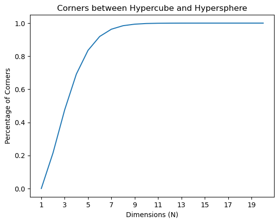
percentage of corners within a hypercube across dimensions
Now this is interesting, as the dimension increases, more and more random points are found in the corners instead of within the hypersphere. After the 9th dimension almost all of the points belongs to the corners. Since our random points are sampled uniformly, we can conclude that as the dimension increases, the spaces within the hypercube seem to have migrated from within the hypersphere to the corners. In other words, the ratio of corners-to-hypersphere increases drastically the higher the dimension goes!
Note that this doesn’t mean that the volume of a hypersphere shrinks monotonically as the number dimension rises. Recall that from earlier calculations the volume of the hypersphere increases from 2D to 3D — We still need to take the exponential volume increase of the hypercube into account.
The Diminishing Hypersphere
We can obtain a rough approximation of the volume of the hypersphere by multiplying the volume of the hypercube ($2^n$) by 1 minus the percentage of corners we got from the previous simulation.
ball_vol = np.array([2**n for n in range(1, N + 1)]) * (1 - corners_percentage)

plt.plot(list(range(1, N + 1)), ball_vol)
plt.title('Estimated Volume of Hypersphere')
plt.xlabel('Dimensions (N)')
plt.xticks(list(range(1, N + 1, 2)))
plt.ylabel('Volume')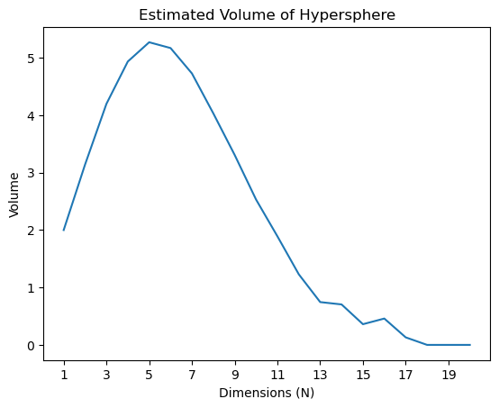
Estimated volume of unit ball across dimensions
For a unit ball (hypersphere with a radius of 1), we can see that its volume peaks around dimension 5, then gradually descends until its volume approaches (but never actually) zero. As it turns out, assuming that a proton takes the shape of a fixed-radius hypersphere, an 11D proton is indeed much smaller than its 2D form!
This is only one of the many counter-intuitive phenomena in the high dimensions.
Now that you’ve learned about the diminishing volume in a hypersphere at high dimensions. Next time your boss tells you to randomly sample points within a high-dimension N-Ball, you will know not to use the rejection method (first sample from the hypercube, then try filtering out the points outside of the hypersphere), as the probability of actually hitting a point within the N-Ball is nearly zero.